From power laws to AI networks, why complex Bitcoin price models memorize market noise

Bitcoin price forecasting has accumulated an unusually colorful collection of methods.

You have basic scarcity models that convert the halving schedule into a price, and run-of-the-mill on-chain models that turn address or transaction activity into value.

The highly contested power-law charts draw an ascending corridor through Bitcoin's history, and machine-learning systems feed market and macroeconomic data into incredibly complex software.

Each of those approaches enters the price-prediction contest against a very shallow, dumbed-down opponent: naive forecasts that use only current market information. A price forecast can use today's price, a return forecast can use zero, and a direction forecast can use a random walk.

Much of the academic literature has struggled to beat it once a model leaves the period in which it was designed.

A May 2026 preprint reviewing Bitcoin prediction research by Carlos Baquero of the University of Porto reached a pretty sobering conclusion: across the peer-reviewed record, no model had demonstrated durable superiority over the appropriate naive benchmark at horizons of one to six months across several market regimes.

The literature contains hundreds of papers, while Baquero selected 23 for close examination based on their methods, influence, or use of genuine out-of-sample evaluation. The review itself is still awaiting peer review, an important distinction when one of its central arguments is that forecasting claims need stronger evaluation.

Short-horizon order flow and daily return forecasts occupy a separate field, and some have produced real predictive value. Online discussions often blend them with longer-horizon price forecasts and valuation models, although each task asks for a different answer.

A formula describing Bitcoin's historical path tells us little about tomorrow's direction, while a daily direction model says little about the price six months from now.

The easiest rival in finance

Naive forecasting works because financial prices are persistent, so a model predicting $100,100 tomorrow when Bitcoin trades at $100,000 today can produce a tiny percentage error even when it has learned almost nothing about direction or return.

Today's price would have been nearly as accurate, and evaluating only the first model gives it credit for information the market had already supplied.

The benchmark becomes more demanding as the horizon expands because Bitcoin can move violently over a month, giving a forecaster room to add value, while the relationships the model learns decay as the market evolves.

A rule calibrated to the retail-led 2017 cycle encountered a different derivatives structure in 2021, and spot ETFs created another route for capital and price discovery in 2024. Each era supplies historical data from a version of the market that no longer exists in quite the same form.

This problem, known as non-stationarity, appears when the relationships between variables don't stay stable enough for past observations to describe the future.

Bitcoin's user base and liquidity have evolved over time, while regulation and access have changed who can trade it and how. A model can capture a relationship during one period and lose it when the market around the asset evolves.

Francesco Puoti, Fabrizio Pittorino, and Manuel Roveri reached a similar result in a study comparing statistical, machine-learning, and deep-learning forecasts. They applied 12 approaches to five major cryptocurrencies at one-day, seven-day, and 30-day horizons.

Simple naive models consistently produced better forecasts than ARIMA, Prophet, random forests, XGBoost, LSTM networks, and N-BEATS.

The result says more about the available information than the sophistication of each method. A complex model can add value when stable patterns exist for it to learn, and it can memorize noise when those patterns are weak or temporary.

Bitcoin offers enormous quantities of data, but the number of independent market cycles it went through is still quite small. Millions of minute bars keep repeating observations from the same 2018 bear market or the same 2020 liquidity shock.

How a backtest becomes a crystal ball for predicting Bitcoin price

Many Bitcoin models look strongest once their creators have seen the entire historical period used to build them. Researchers can try different variables and lookback windows, move the start date, or swap one architecture for another before publishing the best result.

The winner may have discovered a durable relationship, but it also could have won a large lottery conducted on the same price history, an outcome known as backtest overfitting.

David Bailey and his co-authors formalized the problem in their research on the probability of backtest overfitting. Trying more model variations raises the odds of finding an excellent historical result through chance. Selecting the winner and presenting its performance alone hides the number of failed attempts that made the winner possible.

A single chronological split offers little protection because a researcher can train through 2020 and evaluate the model in 2021, producing an apparently out-of-sample result that owes much of its performance to a single bull market.

Walk-forward evaluation is stronger because the model repeatedly retrains on past data and forecasts the next unseen period. Multiple non-overlapping holdout windows are stronger again because they force the same method to encounter bull markets, crashes, sideways periods, and different liquidity conditions.

Among the peer-reviewed papers Baquero examined, none evaluated the same approach across several non-overlapping holdout windows covering different regimes. The strongest papers used rolling or walk-forward evaluation over one continuous out-of-sample period.

Those methods provide real evidence, but a single aggregate error can still hide failure in one section behind success in another.

Information leakage can also lead to false confidence because a feature calculated with future data can give a model a faint view of the answer. You get the same problem when you normalize variables across the full sample, and overlapping return windows can carry future observations across the training boundary.

The error can be subtle enough to survive peer review, especially when a complicated architecture puts several transformations between the raw data and the reported forecast.

The metric itself can flatter the model when a 99% accuracy claim refers to how closely a predicted price level follows the actual price, a relatively easy task for a persistent series.

Traders care about the direction and size of the move, as well as the cost of acting on it. Models that predict $100,500 when Bitcoin moves from $100,000 to $99,500 have a small price error and still make the wrong trade.

The formulas that outlive their forecasts

Bitcoin's best-known valuation frameworks thrive because they turn what's obviously a very complicated asset into a nice, intuitive explanation.

For example, stock-to-flow says scarcity is what drives value, with each halving reducing new supply relative to the existing stock.

Metcalfe-style models say a network becomes more valuable as its user base expands.

The power law says Bitcoin's long history follows a stable mathematical relationship between price and time.

Each of these ideas contains plausible economic intuition, but its forecasting record depends on whether the fitted relationship survives new data and whether simpler explanations account for the same result.

Alexander Shelton's 2024 peer-reviewed examination of Bitcoin return prediction found that stock-to-flow and Metcalfe variables helped explain returns in-sample, but offered limited or zero predictive ability out of sample.

Once time effects entered the stock-to-flow regression, its statistical force disappeared. Bitcoin's supply ratio increases on a predetermined schedule, and its price also climbed for much of its history, making two time-linked series look economically connected.

We saw that weakness in the market long before it appeared in a formal review. The stock-to-flow model diverged from Bitcoin's price as the asset traded below its projected path for years.

Persistent divergence can be absorbed by redefining the output as long-term value or a cycle average, though each redefinition makes the original price claim harder to evaluate.

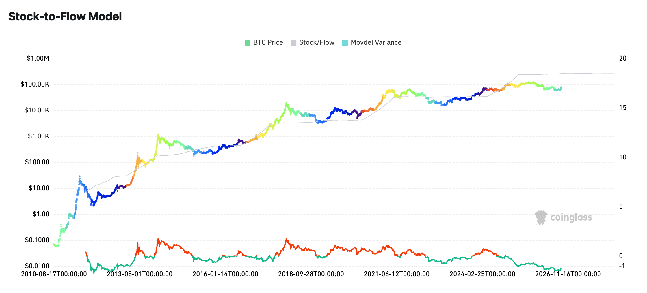Chart compares Bitcoin’s price with the stock-to-flow model and model variance from 2010 through 2026. Source: CoinGlass

Metcalfe's Law faces a related identification problem because network activity and price can climb together when adoption raises value, when a higher price attracts users, or when both variables follow a common time path.

Savva Shanaev and his co-authors used instrumental variables across six proof-of-work assets in a study of mining costs, network activity, and crypto value. Once they addressed autocorrelation and the two-way relationship between activity and price, the positive effects attributed to hashrate and transaction count disappeared.

Power-law models are in a much more complicated position because their corridors have captured much of Bitcoin's historical path and provide a practical visual language for discussing where price lies relative to a long-run curve.

Reports on the Bitcoin power-law model have also shown how ETF-era market structure can alter the forces moving price within that corridor.

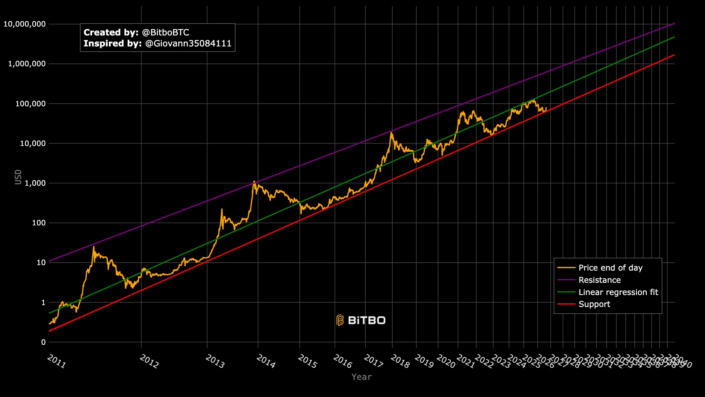Chart plots Bitcoin’s price since 2011 within logarithmic support, resistance and linear-regression bands projected through 2040. Source: Bitbo

The academic issue lies in the strength of the inference. A high R-squared on a log-log chart establishes that a line fits the observed sample. Formal support for a power law also requires evidence about the distribution of residuals and comparisons with other time functions.

Researchers would then need to examine sensitivity to the starting date and performance on future observations. Baquero's review found that the current Bitcoin power-law literature had not yet completed that work.

An honest forecasting standard would publish the naive benchmark beside the model and report every market regime separately. Trading costs belong in the results, while public code and data let other researchers reproduce it.

The paper should also disclose how many variations were attempted, since that number determines how surprising the winning backtest really is. Valuation narratives need to be separated from point forecasts, and the reported range should reflect the asset's uncertainty.

Any correction term should allow a value of zero, letting the model conclude that today's price is its best forecast.

That conclusion will always struggle online because it offers no dramatic target and no date to circle. It has one advantage that the forecast bazaar rarely advertises: it tells us exactly how much the model knows beyond the price already visible to everyone.